Teaching · Computational photonics
Electromagnetic modelling of micro- and nanostructured surfaces
M2 · OIVM master
There is no single numerical method for Maxwell’s equations, only methods matched to a question. Long propagation of a paraxial beam, short propagation around a nanostructure, or no propagation at all when what is wanted is a band diagram: three regimes, three formalisms. The course derives each one from the same starting equations, states the approximation that makes it work, and stops at the point where the student can write the code.
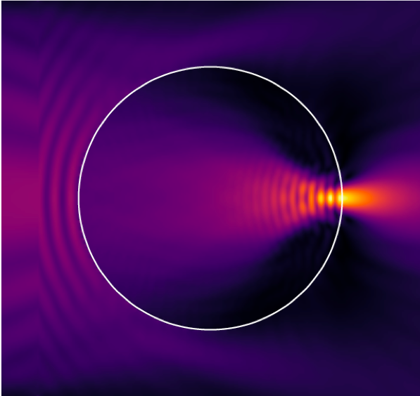
Near field computed around a dielectric cylinder: the quantity the whole course exists to produce.
16 h lectures · 18 h problem classes · Second year of the OIVM master · Course material in English
01What the student takes away
02Course outline
- Positioning: long propagation for short wavelengths, fibres and transport
- Paraxial equation from the monochromatic wave equation
- Slowly varying envelope and Fresnel approximation; loss of polarization
- Diffraction operator D and guiding operator W, Baker-Hausdorff lemma
- Split-step Fourier implementation and its flow diagram
- First implementation: diffraction of a Gaussian beam
- Nonlinear extension: Kerr coefficient and the nonlinear Schrödinger equation
- Positioning: short propagation for short wavelengths, nanophotonics and interaction
- Flow of Maxwell’s equations; linear, isotropic, non-dispersive case
- Time-difference approximation and stable finite-difference equations
- Derivation and anatomy of the update equations, the FDTD algorithm
- Yee grid: unit cell, three-dimensional grids, why not a collocated grid
- Material impedance and normalized magnetic field; curl equations component by component
- Reduction to one dimension, decoupling into two independent modes
- Implementation of the Ey/Hx mode
- In practice: mesh design, time step, boundary conditions, Gaussian pulse source
- Natural and artificial photonic crystals, opals and woodpile structures
- Passive and active devices, integrated optics
- Light scattering: a nineteenth century mystery and its resolution
- Electromagnetism as a Hermitian eigenproblem
- Periodic Hermitian eigenproblem and Bloch modes
- Any one-dimensional periodic system opens a gap
- Two-dimensional TE gap, three-dimensional complete gap
- Unit cell, Brillouin zone, formalism and calculations
03Lecture material
Three sets of slides, one per method. Each one carries the derivation and the corresponding code fragments, so that the implementation is never separated from the equation it discretizes.
04Problem classes
Eighteen hours at the keyboard, five sheets following the three methods in order. Each block ends on an open question that has no analytical answer, handed in as a short set of slides together with the code.
The split-step Fourier scheme built from scratch and checked on a case whose answer is known, then pointed at an experiment that has none.
- Build the (x, y) grid and the conjugate (kx, ky) grid required by the Fourier implementation
- Generate the initial Gaussian field, waist w0 = 50 µm at λ = 1.03 µm
- Apply the thin lens phase mask, f = 10 mm, and verify energy conservation before and after propagation
- Propagate with the Fresnel transfer function up to Zmax = 30 mm; transverse intensity at the lens and at Zmax
- Track the beam width along z, where the amplitude drops to 1/e of its maximum
- Extension: index map n(x, y, z) of a single silicon cone, 5 µm base tapering to 1 µm over a height of 10 µm, standing in a 10 µm pool
- Propagate the transmitted field in air up to 200 µm above the tip, plot a longitudinal (x, z) cut, and explain the ring seen in the measurements
The update equations of the lecture turned into a running code, then confronted with an interface.
- Domain of 5 µm sampled with N = 1001 points, time step set by the Courant number, 2000 iterations
- Ex polarized along x, Hy along y, propagation along z; coefficients ae, am and as for a medium of conductivity σ
- Point source, Gaussian in time, λ = 800 nm, half width at 1/e of 15 fs
- Propagation in vacuum, then reflection on sharp and on smooth index transitions
The open part of the FDTD block: a 300 by 300 grid, a real material, and a number at the end rather than a pretty map.
- Pulse Gaussian in time (10 fs) and in space (5 µm) at λ = 800 nm, perfectly matched layers at the boundaries
- Propagation in vacuum: decide whether an Ex component appears, and say why
- Tungsten layer 100 nm thick, n = 3, σ = 5 × 10⁵ S/m at 800 nm, then a Drude model for a realistic dispersion
- Surface morphologies on the tungsten (bump, spike, rod, hole, interacting or periodic) and the local field enhancement they produce
- Field enhancement factor against the geometrical parameters, and absorption cross-section from the Poynting flux
The stationary problem, where propagation is replaced by an eigenvalue calculation.
- Unit cell of two layers: l1 = 200 nm with ε1 = 1, l2 = 800 nm with ε2 = 9
- Fourier expansion of 1/ε(x) on N = 2 numG + 1 plane waves, with numG = 50
- Analytical expansion coefficients, matrix differential operator, band structure across the Brillouin zone
The same formalism in two dimensions, on a lattice whose gaps have to be opened by hand.
- Square lattice first, then the band structure of a hexagonal lattice with r = 20 nm and a = 75 nm
- Arrays of voids: effect of the permittivity contrast on the gaps
- Projection of the complete photonic band gap as a function of r/a
- TE and TM polarizations compared, and the role of the dielectric contrast for each
Note
The course was previously listed under the title Nanophotonics. Slides are in English.

